Le role de la paille dans la correction acoustique - CFA 14 ème Congré Français d'Acoustique
The role of straw in acoustic correction
Maitre assistante A Université de Constantine 3, Algérie
Author: Farid Dalal
Author: Farid Dalal
| View Paper |
Noise Pollution Shield System for Pedestrians for Coach Termini/Stops in Hong Kong
Design Strategy for a new Generic Environmental “Shield” as Bus Stops
School of Architecture, The Chinese University of Hong Kong, April 22nd 2016
Author: Fernando Nohrá Castro
Author: Fernando Nohrá Castro
|
| ||||
Revisiting the Schroeder Frequency: The Influence of Room Proportions and Subsequent Modal Distributions on the Validity of the Schroeder Cutoff Frequency
Department of Audio Arts and Acoustics, Columbia College Chicago
Author: Gordon M. Ochi
Author: Gordon M. Ochi
| View Paper |
Traffic Noise Assessment Comparing Two Modeling Tools: Traffic Noise Model 2.5 & Olive Tree Lab
Columbia College Chicago: Audio Arts and Acoustics
Author: Isabel Garcia
A comparison between Traffic Noise Model (TNM) provided by the Federal Highway Administration and Olive Tree Lab Suite. The results of TNM and OTL were compared to actual test data acquired from on-site testing.
Author: Isabel Garcia
A comparison between Traffic Noise Model (TNM) provided by the Federal Highway Administration and Olive Tree Lab Suite. The results of TNM and OTL were compared to actual test data acquired from on-site testing.
| View Poster |
The Significance of Sound Diffraction Effects in Predicting Acoustics in Ancient Theaters
This project examines, sound diffraction effects at the steps of ancient theatres and how significant these effects are in predicting their acoustical properties. In order to examine the significance of such effects, sound measurements were taken at the ancient theatre of Kourion in Cyprus. These measurements were then compared to simulations by modelling Kourion in OTL – Terrain which also handles sound diffraction to high orders. Sound measurements at Kourion were the apex of a series of preparatory work since the place is a monument, and the effort was to secure valid measurements during one visit only. In order to validate both hardware and software to be used in the final Kourion measurements, sound measurements were taken inside Cyprus University of Technology semi-anechoic chamber prior to the Kourion measurements. The Kourion measurements scenario was “rehearsed” at Heritage school theatre, a recently built open theatre in the fashion of ancient Greek theatres.
More in-depth information can be found below:
More in-depth information can be found below:
Semi-anechoic chamber at cyprus university of technology
Preparatory Work at CUT Semi Anechoic Chamber
Introduction
Olive Tree Lab Terrain’s calculation results had been validated, before this project began, based on further scientific findings. In order to validate the accuracy of OTL – Terrain, we carried out measurements at the Cyprus University of Technology semi-anechoic chamber. Furthermore, in anticipation of a complex sound transfer function from sound measurements at Kourion, we used the semi-anechoic measurements to discover the “signature” of diffraction from a step-like structure.
Olive Tree Lab Terrain’s calculation results had been validated, before this project began, based on further scientific findings. In order to validate the accuracy of OTL – Terrain, we carried out measurements at the Cyprus University of Technology semi-anechoic chamber. Furthermore, in anticipation of a complex sound transfer function from sound measurements at Kourion, we used the semi-anechoic measurements to discover the “signature” of diffraction from a step-like structure.
|
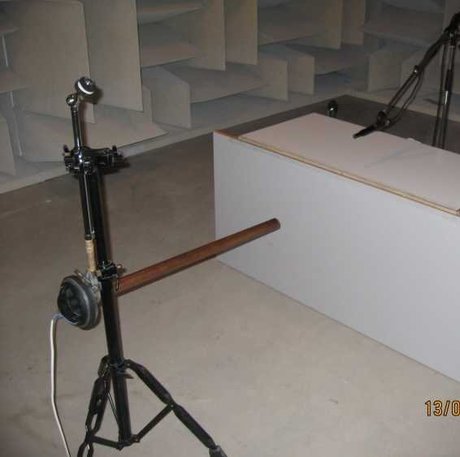
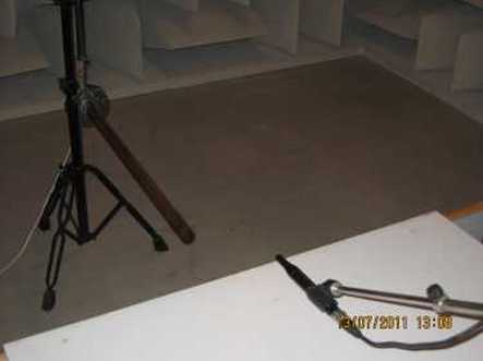
Figure 1. Measurements at the semi-anechoic chamber of the Technological University of Cyprus. Omnidirectional source, microphone and step-like barrier can be seen.
|
Objectives
- Validate OTL – Terrain’s results.
- Exercise and evaluate the acoustic measurement software setup parameters.
- Validate the hardware used during the sound measurements.
Measurements Procedure
Instrumentations used
Instrumentations used
- Laptop with WinMLS acoustic measurement software application and sound card
- Omnidirectional source consisted of a 1,5’’ horn driver with 70cm tube attached (ANSI S1.18-2010)
- 90 Watt stereo amplifier for the Omnidirectional source
- Preamplifier for the microphone
- NTI MiniSPL Class 2, Omnidirectional microphone
- Step-like barrier made of smooth wooden surfaces
|
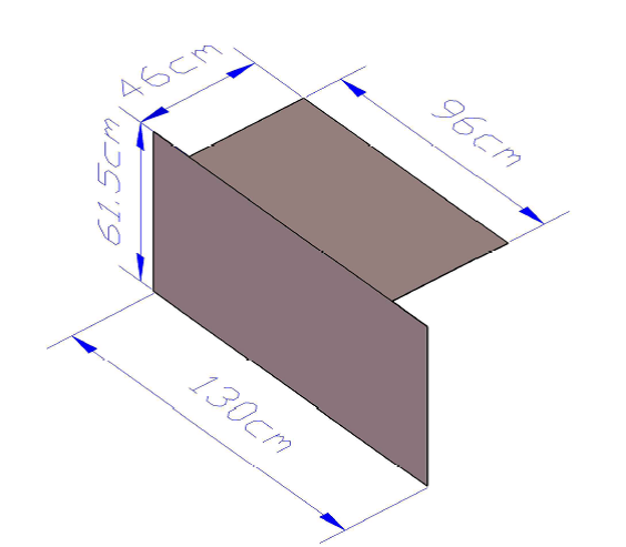
Figure 2. The CAD drawing of the step that was used as a sound barrier in the semi-anechoic chamber
|
This step-like structure was used to set up four different configurations inside the semi-anechoic chamber. The configurations are presented in the following table and are available for download as OTL – Terrain Projects.
Table 1. The five configurations created in the semi-anechoic chamber
|
The omnidirectional source was fed with sine sweep signal ranging from 1000 Hz– 24000 Hz.
|
|
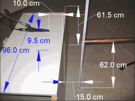
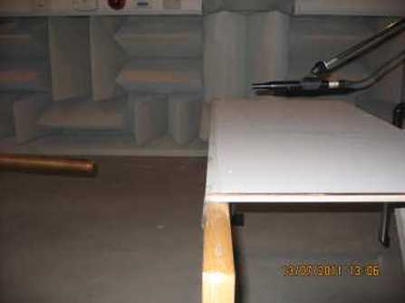
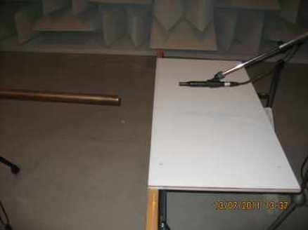
Figure 3 and 4. Photographs of one of five set ups examined in the hemi-anechoic chamber including description of the source, microphone and object distances and dimensions. On the left, the set up with the step like structure and on the right without it
|
|
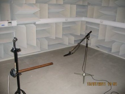
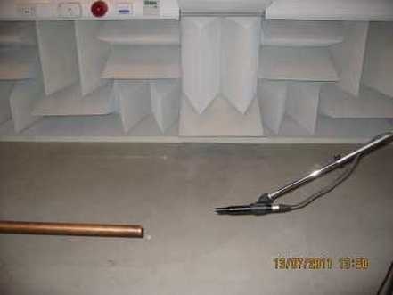
Figure 5 and 6. Step, source and receiver in the semi-anechoic chamber.
At the 4th and 5th configuration the source’s and receiver’s heights don’t change, but the 5th configuration has no barrier. Therefore we can compare the results before and after inserting the barrier, extracting the Insertion Loss (IL) of the barrier or the Excess Attenuation (EA)
|
|
Figure 7 and 8. At the left: configuration 4 with barrier. At the right: configuration 5 without barrier.
Horn Driver as a Source - Limitations
After examining the anechoic results, it became evident that there was wave interference at the receiver due to diffraction effects at the rim of the horn driver body. Thus, not only was the time window limited to pick up only the step edge contribution, but it was also limited to prevent diffraction effects from the driver.
After examining the anechoic results, it became evident that there was wave interference at the receiver due to diffraction effects at the rim of the horn driver body. Thus, not only was the time window limited to pick up only the step edge contribution, but it was also limited to prevent diffraction effects from the driver.
Results
Hemi-anechoic Chamber Results
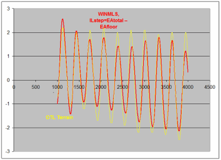
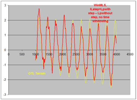
All set ups were calculated in OTL - Terrain and measurements and simulations show a good agreement. However, the agreement between measurements and simulations in the calculation of the Insertion Loss of the object (ILstep=EAtotal – EAfloor = Lpwith step – Lpwithout step), by two independent procedures supports even more the validity of Olive Tree Lab-Terrain prediction power. In the first procedure, the sound pressure level (SPL) is measured with and without the object for a fixed S and R set-up. Their level difference gives IL. Alternatively, the difference between EAtotal and EAfloor (both with step extracted from measurements) and the calculated IL from OTL-Terrain yields the same results (without having to move any objects). The figure below on the left shows a comparison of the IL between measurements and calculations with and without the step in place, while figure on the right, shows the same results with the step in place. The receiver is in the illuminated zone.
The OTL – Terrain Project files, drawing and other information is available here for download.
Hemi-anechoic Chamber Results
All set ups were calculated in OTL - Terrain and measurements and simulations show a good agreement. However, the agreement between measurements and simulations in the calculation of the Insertion Loss of the object (ILstep=EAtotal – EAfloor = Lpwith step – Lpwithout step), by two independent procedures supports even more the validity of Olive Tree Lab-Terrain prediction power. In the first procedure, the sound pressure level (SPL) is measured with and without the object for a fixed S and R set-up. Their level difference gives IL. Alternatively, the difference between EAtotal and EAfloor (both with step extracted from measurements) and the calculated IL from OTL-Terrain yields the same results (without having to move any objects). The figure below on the left shows a comparison of the IL between measurements and calculations with and without the step in place, while figure on the right, shows the same results with the step in place. The receiver is in the illuminated zone.
The OTL – Terrain Project files, drawing and other information is available here for download.
|
|
Figures 9 and 10. On the left: comparison of the IL between measurements and calculations with the step in place. On the right: comparison of the IL between measurements and calculations with and without the step in place.
The following graph represents a comparison between measurements and calculation results for configuration 2. The receiver is in the shadow zone.
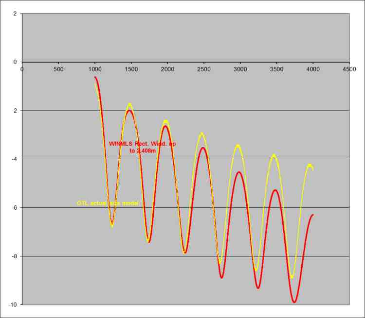
Figure 11. Excess Attenuation (EA) results. Yellow curve represents the EA calculated in OTL-Terrain. Red curve represents the EA extracted from measurements.
General Methodology
This graph proves that OTL-Terrain’s results are valid. The files needed in order to reproduce these results are available for download. Below is described the method used to extract Total Excess Attenuation (EA) from measurements and OTL – Terrain:
Below is described the method used to extract IL (Insertion Loss) from measurements and OTL–Terrain.
This graph proves that OTL-Terrain’s results are valid. The files needed in order to reproduce these results are available for download. Below is described the method used to extract Total Excess Attenuation (EA) from measurements and OTL – Terrain:
- Use “REFERENCE hs=62, hr=71, d=25, no barrier meas 4.wav”, as your reference measurement of direct sound, excluding diffraction effects, from tube horn driver by applying a rectangular window just before diffraction effects, i.e. from 0 – 1.663m. The distance between S & R = 0.266m.
- Use “Anechoic Step 1, hs=62, hr=71, xs=15, xr=10, hb=61.5 meas 5.wav” measurement and apply a rectangular window to exclude the tube horn driver diffraction effect (see Anechoic EAnew(EAnew=IL+EA), hs=36, hr=71 d=25 OTL vs Measurements.xls for each measurement settings).
- Export data into Excel.
- Export from OTL Terrain IL + EA into Excel and add them.
- Measure distance of 1st path (direct or diffracted) from OTL Terrain for distance correction and apply 20log*(0.266/1st path dist.) to the measurement exported data.
- This should give you EA-new which should match OTL Terrain and measurements.
Below is described the method used to extract IL (Insertion Loss) from measurements and OTL–Terrain.
- Subtract with barrier from without barrier measurement, (Anechoic Step 1, hs=62, hr=71, xs=15, xr=10, hb=61.5 meas 5.wav & REFERENCE hs=62, hr=71, d=25, no barrier meas 4.wav), by setting the last one as a reference measurements. No special window applied. A rectangular window was used from 0 – 8m, where there is a smooth response.
- Export data into Excel.
- Export from OTL Terrain IL into Excel and add them.
Conclusions
OTL Terrain was tested and validated for its results by comparing them with actual measurements.
OTL Terrain was tested and validated for its results by comparing them with actual measurements.
Heritage school amphiTheatre
Preparatory Work at Heritage School Theatre
Introduction
Sound measurements were conducted at the Heritage school theatre, a recently built open theatre in the fashion of ancient Greek theatres. This allowed a rehearsal of the acoustic measurements that would be performed later at the ancient theatre of Kourion.
Sound measurements were conducted at the Heritage school theatre, a recently built open theatre in the fashion of ancient Greek theatres. This allowed a rehearsal of the acoustic measurements that would be performed later at the ancient theatre of Kourion.
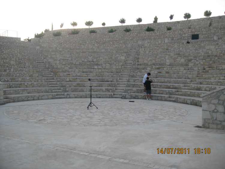
Figure 1. Heritage School Theatre. (At the centre of the orchestra the omnidirectional source is positioned at a height of 1.5 m.)
Objectives
- Exercise and evaluate the acoustic measurement software setup parameters.
- Exercise and evaluate theatre imprinting method.
- Exercise and evaluate the microphone positioning method.
- Determine the type of source to be used for the measurements.
- Determine the post processing procedure for the measurement analysis and get preliminary results to compare with calculations.
- Measure evidence to support the ray equivalency theorem.
Measurements Procedure
Instrumentation
Instrumentation
- Laptop with acoustic measurement software application and sound card
- Two way 10” active constant directivity speaker unit
- Omnidirectional source consisted of a 1,5’’ horn driver with 70cm tube attached (ANSI S1.18-2010)
- 90 Watt stereo amplifier for the Omnidirectional source
- Preamplifier for the microphone
- NTI MiniSPL Class 2 Omnidirectional microphone
- Portable weather station
Three positions were specified to be measured, on three different steps of the theatre, 1st, 7th and 14th. Here are the OTL – Terrain Project files with theatre equivalent and the three receiver positions. In order to create a detailed 3D model in OTL Terrain, additionally to using the theater’s architectural drawings, we measured the dimensions of all steps in the cavea.
The idea was to take dimensions and acoustic measurements on two different rays over the cavea from the centre of the orchestra.
The idea was to take dimensions and acoustic measurements on two different rays over the cavea from the centre of the orchestra.
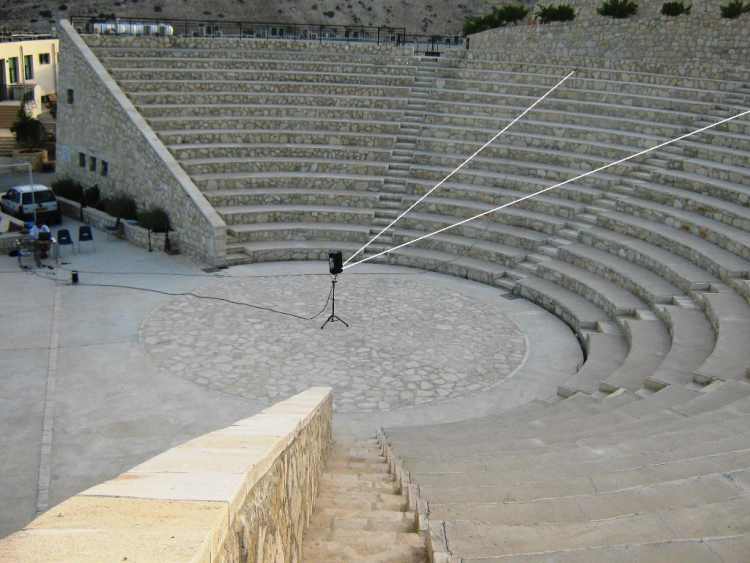
Figure 2. The two lines represent the rays over the cavea where measurements were conducted in order collect evidence to verify the ray equivalence theorem.
For the acoustic measurements, we initially defined the source’s and the receivers’ location by measuring with a measuring tape.
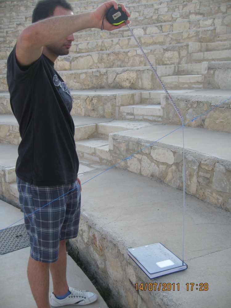
Figure 3. Measuring the microphone position on the first step. The blue string defines the section line over the cavea on which sound measurements were conducted.
The source was placed in the orchestra’s centre at a height of 1.5m. To define the center of the orchestra, the distance from centre to any point of the first step’s forehead surface was measured to be equal to 6.25m.
|
|
Figure 4. The omnidirectional source consisted of a 1.5’’ compression driver with 70cm tube attached (ANSI S1.18-2010), placed in the centre of the orchestra at 1.5m height.
The cavea is divided by columns of smaller steps for audience movement up and down the theatre. Sound measurements eventually were taken at the centre line between two steps-columns at a height where an audience would be seated (75cm), above the edge of 3 steps. Those 3 steps are the 1st (closest to the orchestra), 7th and 14th.
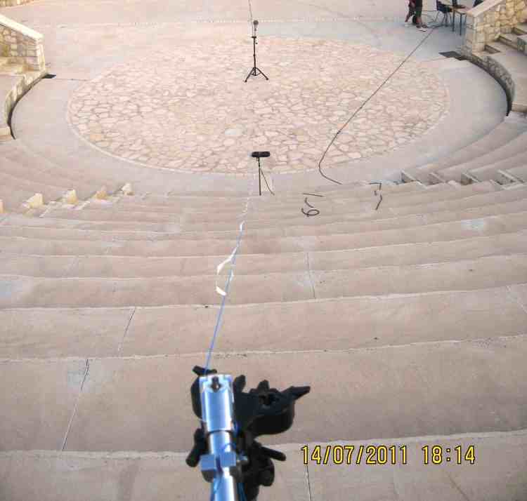
Figure 5. The measurements at the 2nd section line over the cavea
We measured the impulse response at the 3 receivers’ locations mentioned above, using sine sweep signal ranging from 1000 Hz– 24000 Hz. We repeated the measurements using the 2-way active speaker as a source. The sine sweep signal range was changed to 70 – 24000 Hz.
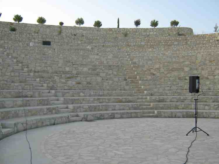
Figure 6. The 10’ active speaker positioned at the centre of the orchestra at a 1.5m height, taking into consideration the acoustic centre the 10’ cone driver
Following the same procedure, measurements were also taken at a different section line of the theatre, in order to verify the Ray Equivalence Theorem.
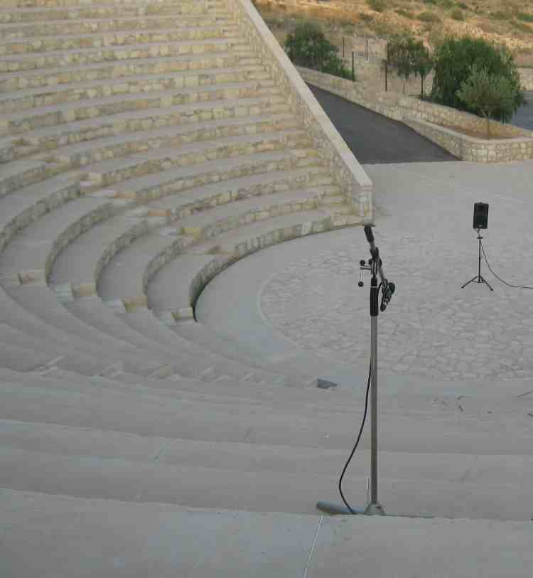
Figure 7. The measurements at the 2nd section line over the cavea
The OTL – Terrain Project files, drawing and other information is available here for download
Results
The EA was extracted from the measurements and compared to OTL– Terrain results. (Information about the methodology can be found here). Good agreement was found in order to go forward with the measurements in Kourion.
The EA was extracted from the measurements and compared to OTL– Terrain results. (Information about the methodology can be found here). Good agreement was found in order to go forward with the measurements in Kourion.
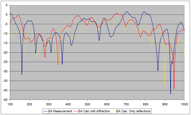
Figure 8. EA is plotted vs frequency. The blue and red curves are the measured and calculated respectively. The yellow curve represents calculation conducted only with reflections
Another result of the analysis was the verification of the equivalence theorem.
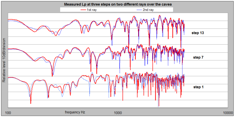
Figure 9. SPL for the three steps measured. Red and blue curves are the results from the measurements along the two different rays over the cavea from the centre of the orchestra.
Conclusions
- Measurements with active speaker were in good agreement to calculated results.
- The use of the omnidirectional source was rejected because of significant interference issues due to the shape of the source.
- The use of a measuring tape to measure distances, especially to locate the position of the microphone in the cavea was not accurate enough.
- Equivalency theorem was verified
- Setup parameters were defined for measurements at the Kourion Theatre.
Kourion Ancient Theatre
Measurements at the Ancient Theatre of Kourion
Introduction
After preparatory work at the semi-anechoic chamber and the Heritage school open theatre, all necessary procedures on source – receiver positioning, measurements parameters and post processing methodologies were finalized in order for us to conduct the crucial sound measurements at the ancient theatre of Kourion.
After preparatory work at the semi-anechoic chamber and the Heritage school open theatre, all necessary procedures on source – receiver positioning, measurements parameters and post processing methodologies were finalized in order for us to conduct the crucial sound measurements at the ancient theatre of Kourion.
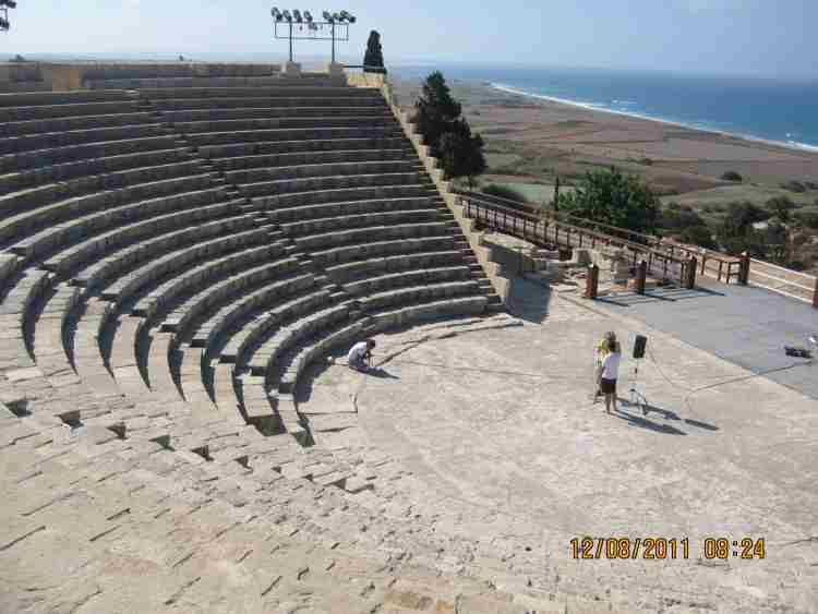
Figure 1. Ancient theatre of Kourion with cavea, orchestra and smaller steps tagged.
Objectives
- Measure in detail the dimensions at a section of the ancient theatre of Kourion
- Complete sound measurements at 35 receivers, in the Kourion audience area, at 38,5cm distance from each other.
- Simulate the Kourion theatre acoustic behavior
- Compare the simulation results vs. measurements
Measurements Procedure
Imprinting of the ancient theatre of Kourion
The accuracy of the design of the theatre, which is needed for the acoustic simulation, has a great effect on the outcome of the results. Therefore, the detailed imprinting of the space is very significant.
Imprinting of the ancient theatre of Kourion
The accuracy of the design of the theatre, which is needed for the acoustic simulation, has a great effect on the outcome of the results. Therefore, the detailed imprinting of the space is very significant.
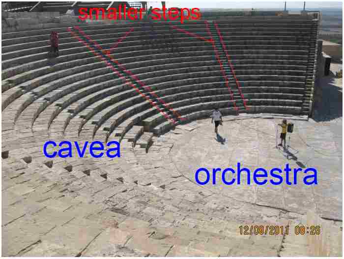
Figure 2. Ancient theatre of Kourion with cavea, orchestra and smaller steps tagged.
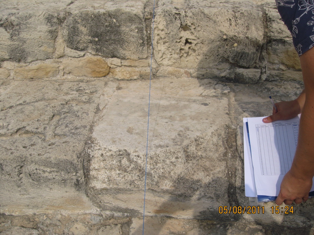
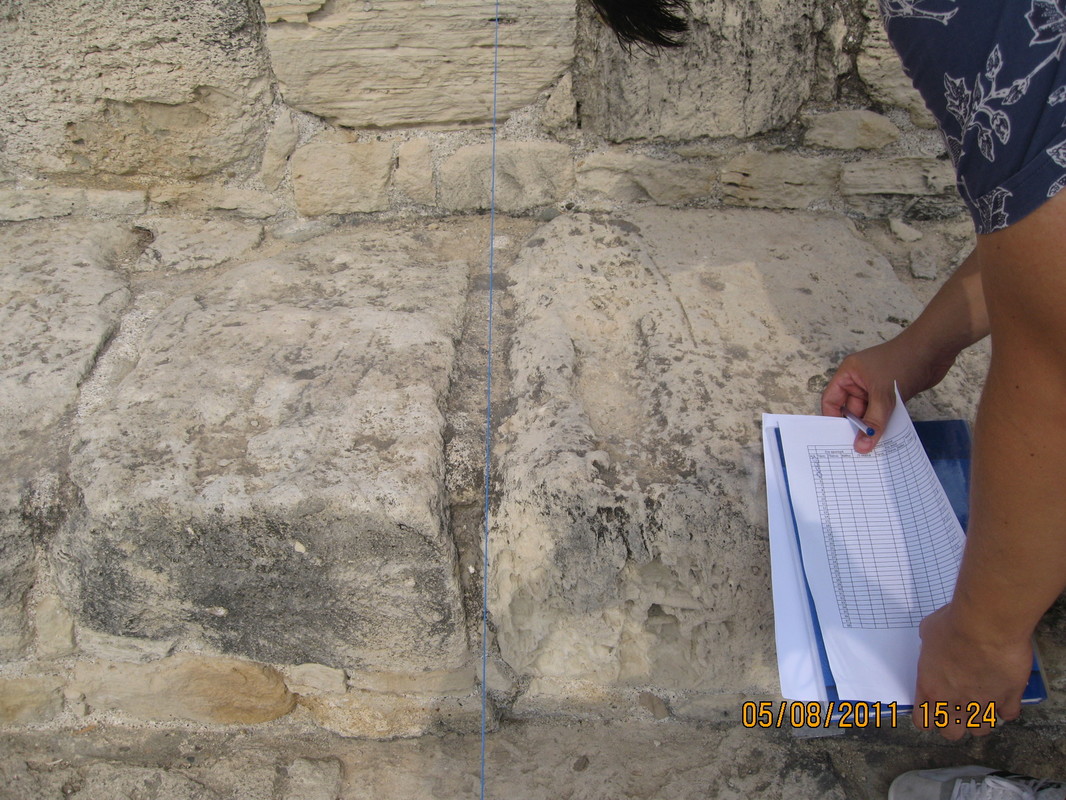
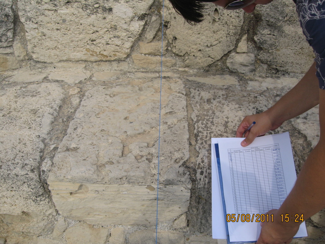
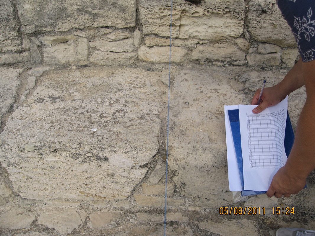
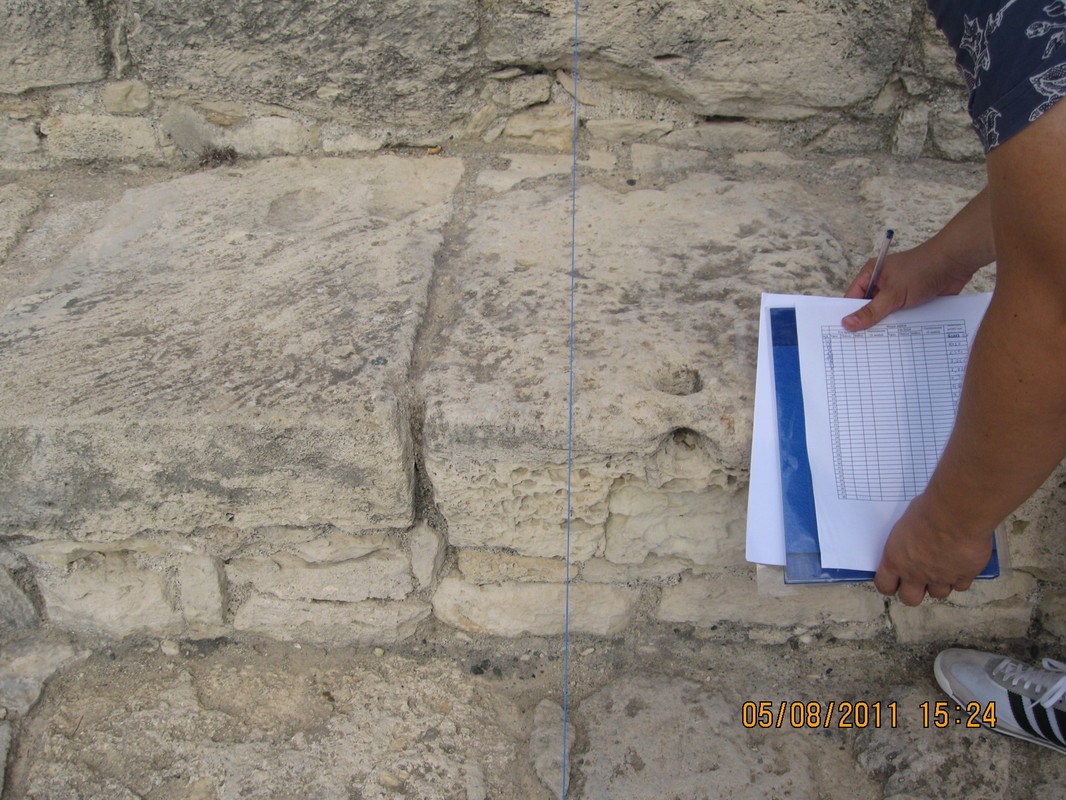
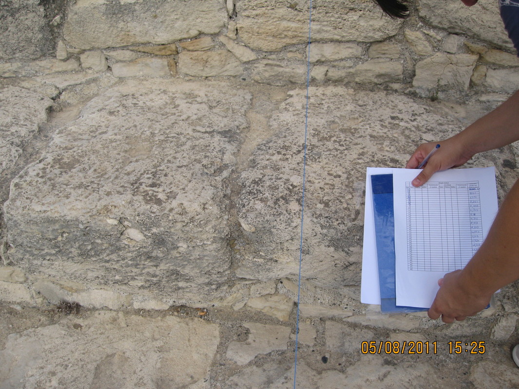
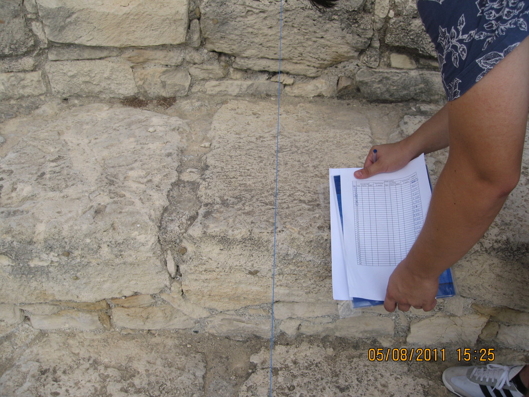
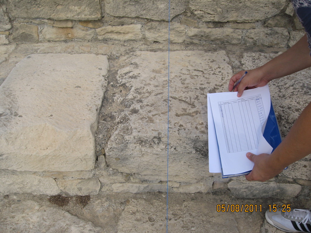
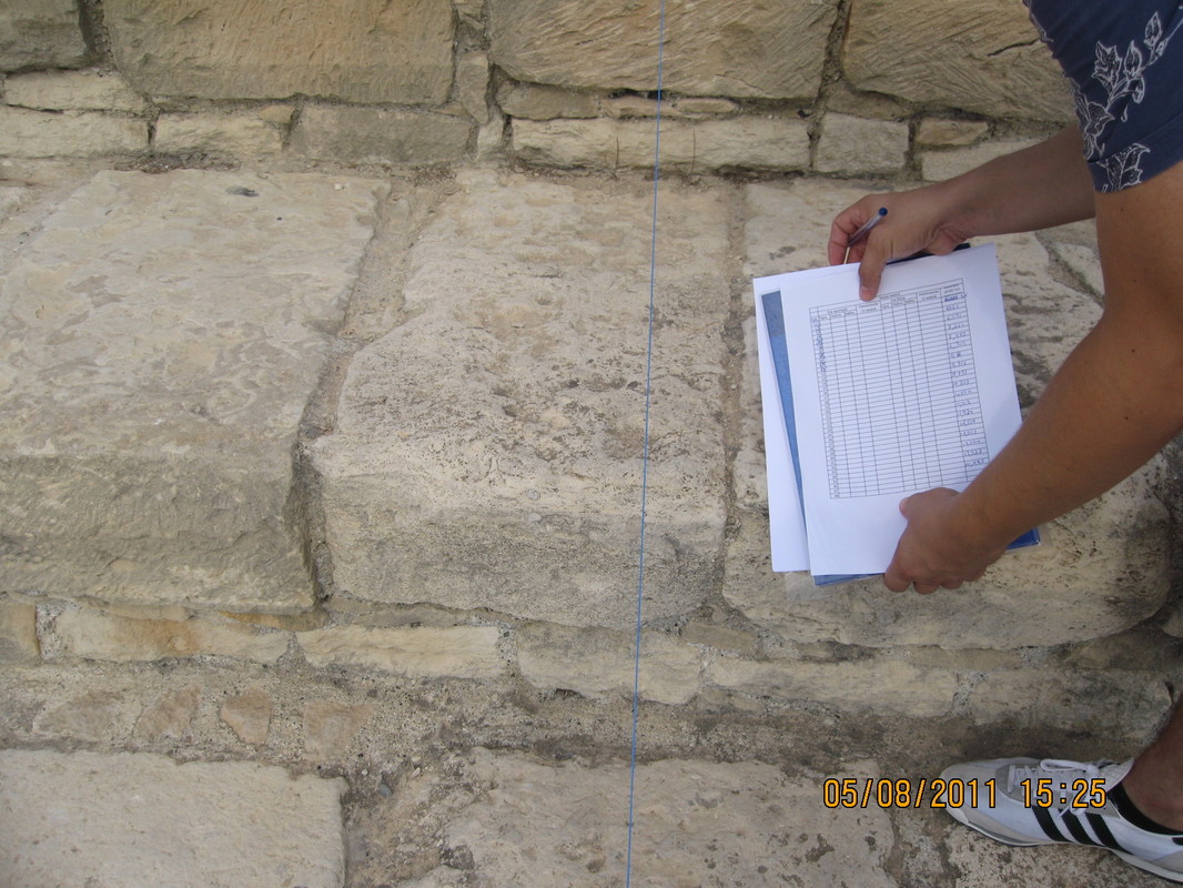
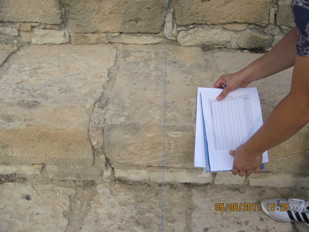
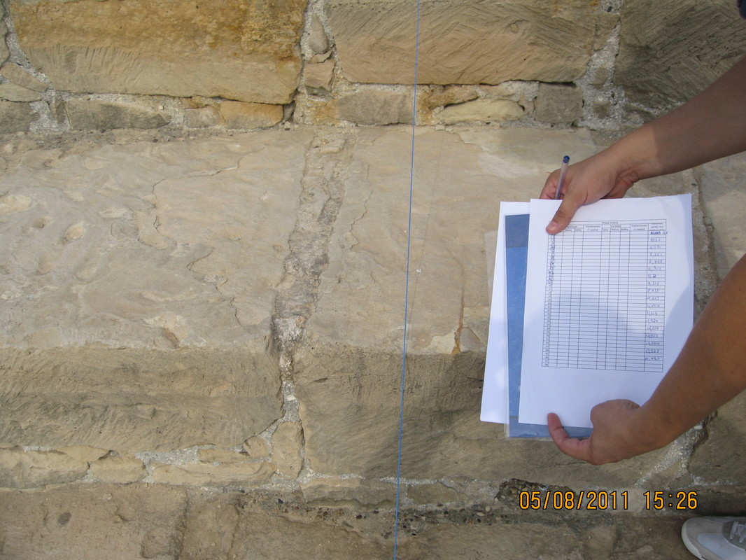
After studying the cavea area of the theatre, we concluded that the section of the theatre and more specifically, the imaginary line, on which the acoustic measurements will be taken, would be on the eastern cavea. First, we defined the exact center of the orchestra and then we measured the orchestra’s radius. The auditorium area of the theatre is separated by columns of smaller steps. The acoustic measurements would be taken along the middle of these steps. Based on this, we measured the distances between the 2 continuous smaller steps, indicated in the above figure, on each row of seats and we placed a marker on the middle of each measured distance. The imaginary line, that connects all of the markers, starting from the center of the orchestra and ending at the middle of the 2 smaller steps of the last row of seats, indicates where the necessary dimensions will be measured.
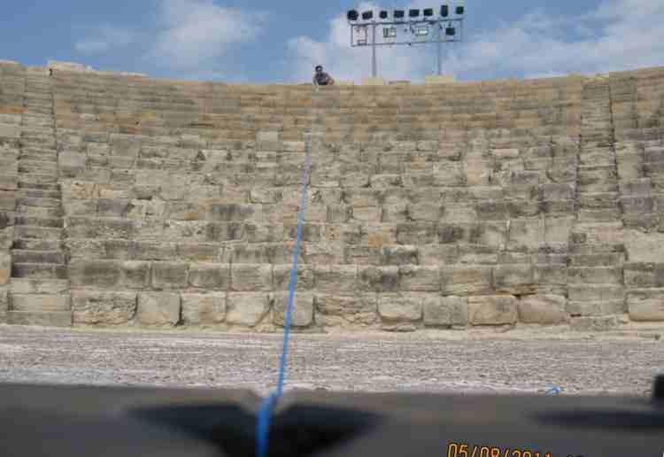
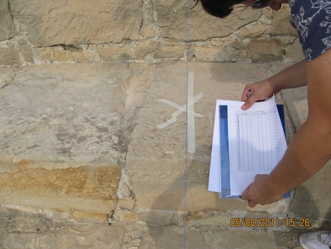
Figure 3. A blue string is placed in the middle between the columns of the smaller steps in the east section of the cavea, indicating the location where the dimensions of the cavea will be measured.
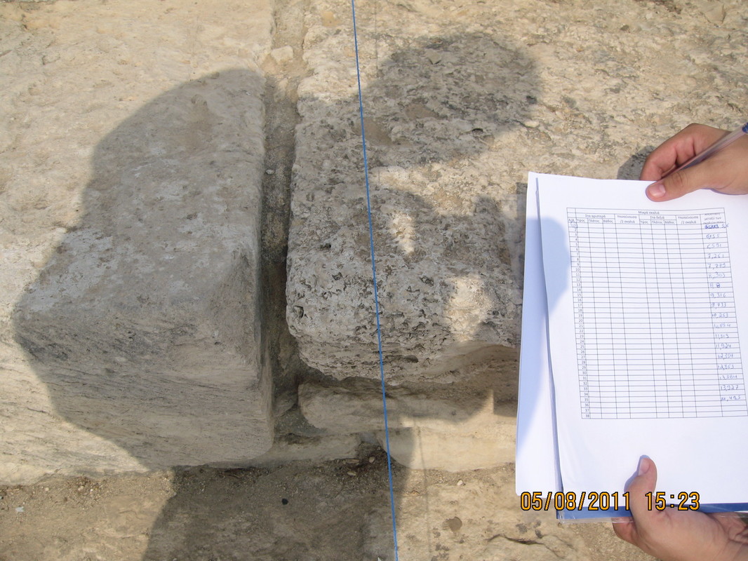
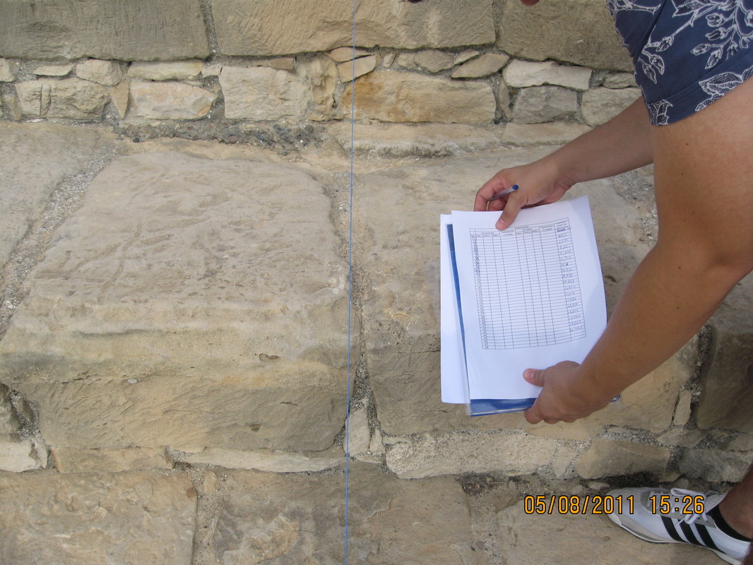
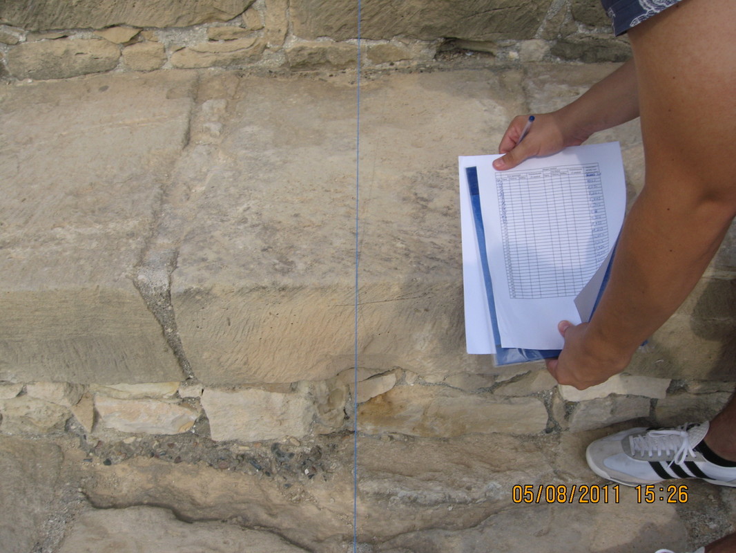
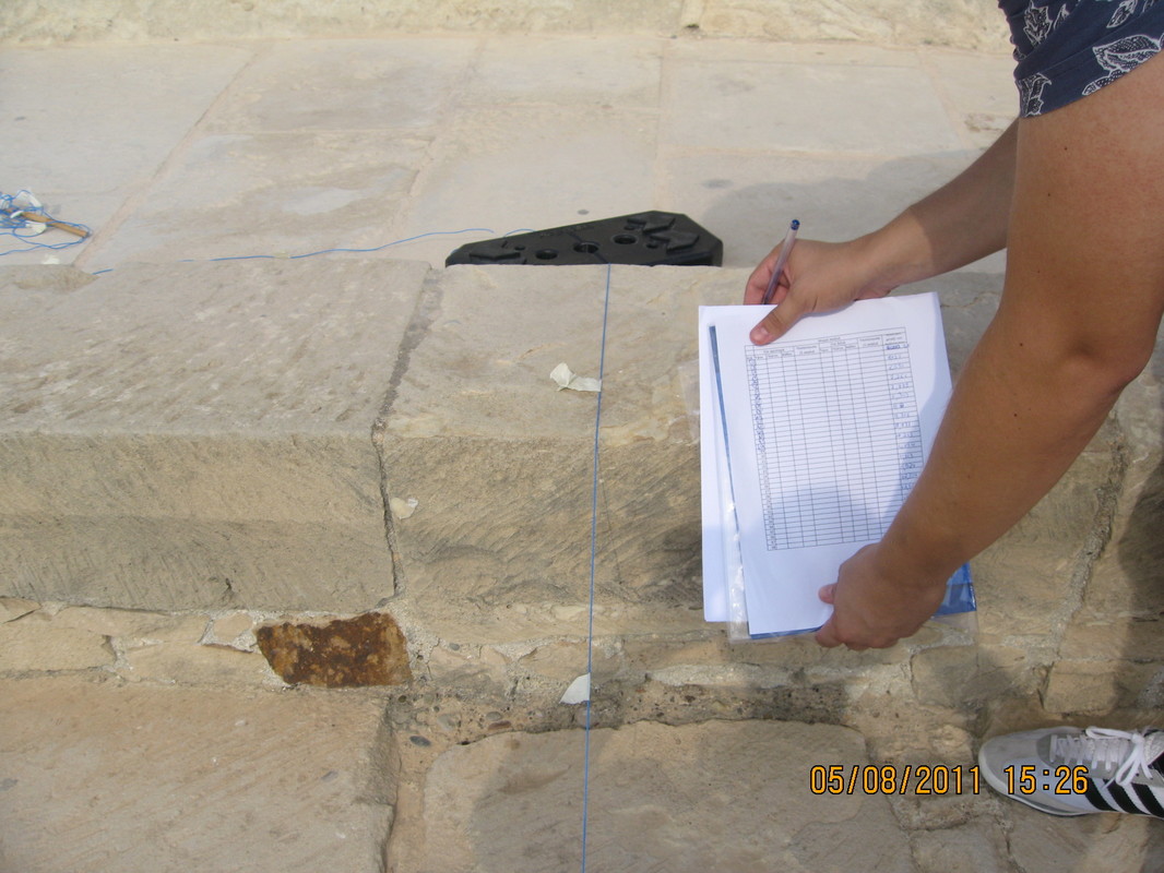
Each step’s surfaces’ dimensions were measured individually, by the use of a laser distance meter. Specifically, the following 4 dimensions were taken at each step:
- The depth from the edge of the step to the extension of the edge of the upper step.
- The entire depth of each step.
- The height of the step, measured from the preceding step to the beginning of the vertical side of the current step's forehead.
- The height of the step measured from the preceding step to the edge of the current step
Additionally, the slope of each step’s planar surface was taken using a laser distance meter.
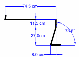
Figure 4. Dimensions measured at the 13th step. The angle, shaped by the preceding step’s planar surface and the 13th step’s sloping surface, was calculated from the measured distances
The measured distances were used to create the 3D model of the theatre in AutoCAD2010 software application.
|
|
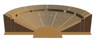
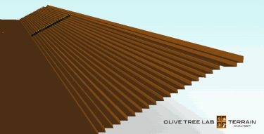
Figure 5. On the left a model of Kourion (as it was originally built) and on the right, the equivalent model used in the simulations.
We photographed each step separately for later reference. Furthermore, knowing each step’s geometry was helpful in the analysis of the acoustic measurements:


Acoustic Measurements at the Ancient Theatre of Kourion
The ancient theatre of Kourion is a historic monument; therefore, it imposes specific permissions in order to perform actions such as acoustic measurements. Furthermore, the theatre receives hundreds of visitors every day, between the hours of 9:30am and 17:30pm. Therefore, the available time for the acoustic measurements is limited. The least windy time of the day in the area of Kourion is during the early hours of the morning, when temperatures are low. Consequently, all these restrictions led us to conduct the acoustic measurements very early in the morning.
Prior to our visit to the theatre for the acoustic measurements, the exact positions where the microphone would be placed was estimated using a 3-dimensional drawing of the theatre. Additionally, we predetermined the position, slope and heading of the laser distance meter that would assist us in taking the measurements.
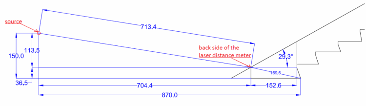
Figure 6. The exact position of the laser distance meter
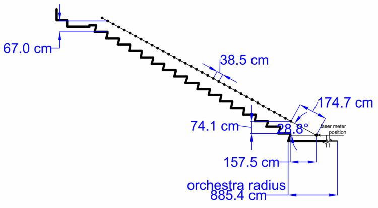
Figure 7.The locations of the 35 receivers above the cavea. Microphone positioning along the section line over the cavea was in increments of 38,5cm
Here are available for downloading the OTL – Terrain Project files with theatre equivalent and the 35 receiver positions.
Instrumentation used:
Instrumentation used:
- Laptop with acoustic measurement software and sound card
- Two way 10” active constant directivity speaker unit
- Preamplifier for the measurement microphone
- NTI MiniSPL Class 2 Omnidirectional microphone
- Portable weather station
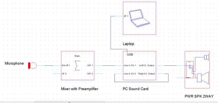
Figure 8. Schematic of the audio equipment connections
Measurements Procedure
Initially, we placed the laptop and the other equipment at a range where minimum interference would occur.
Initially, we placed the laptop and the other equipment at a range where minimum interference would occur.
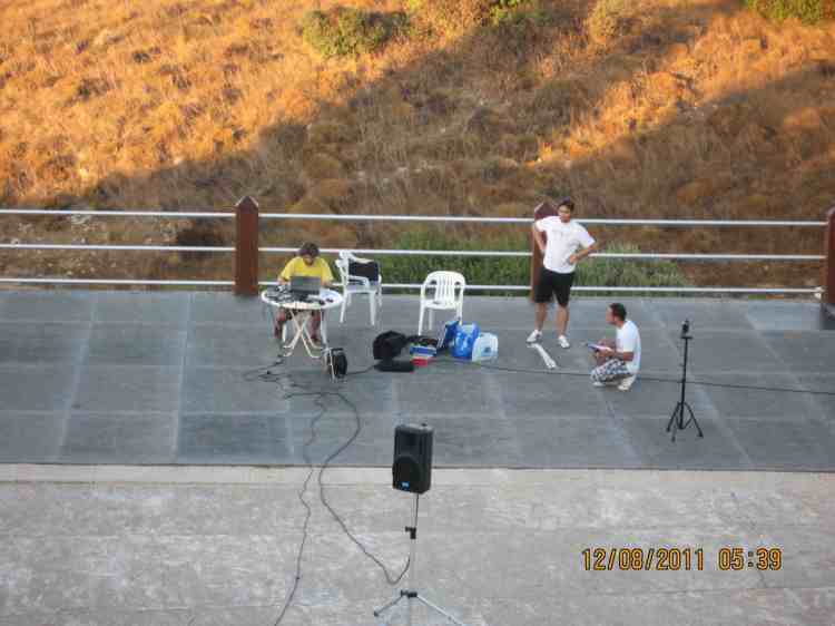
Figure 9. Laptop and preamplifier placed at the furthest possible position from source and receiver
We placed the source, as in Heritage Theatre configuration, in the centre of the orchestra at a height of 1.5 m.
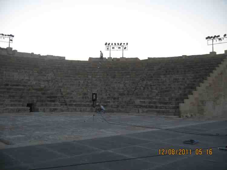
Figure 10. Source positioned at the centre of the orchestra. Center was verified by measuring the radius from the center to the first step
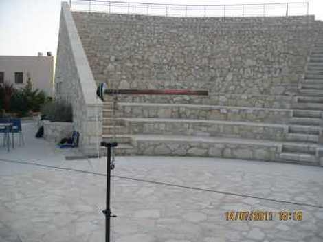
The laser distance meter was placed to the predefined steady position in the orchestra and directed its ray on the imaginary section line of measurement. The lines average height was 75cm above each step’s edge.
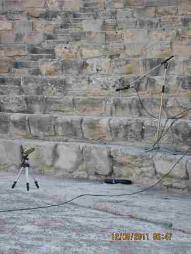
Figure 11. The laser distance meter as it was placed in the orchestra
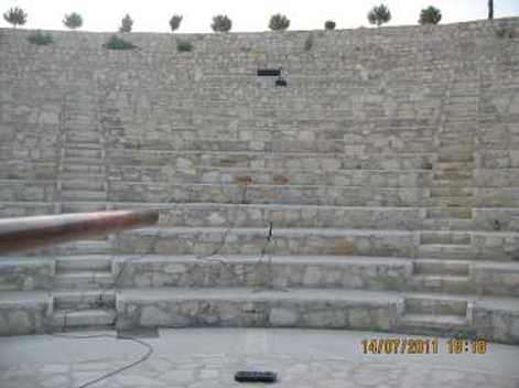
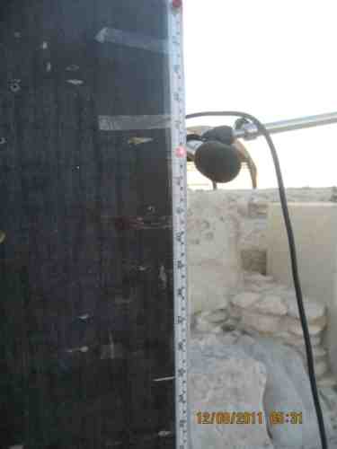
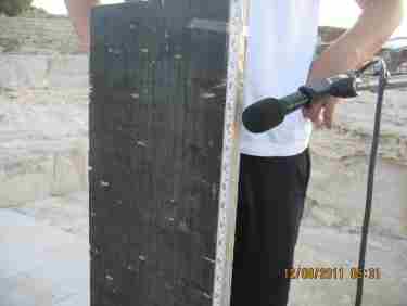
We placed the 2-way active speaker at the centre of the orchestra. The location of the first receiver was found by placing a surface vertically on the first step and moving it to the point where the laser meter would indicate a distance of 175cm. The point where the laser’s ray met the surface indicated the place where the microphone should be placed.
Moving the surface backwards, in order to increase the distance from the laser by 38.5cm, the position of the second receiver was found. We repeated this procedure for 35 receivers. Moreover, directing the laser distance meter to the east evoked a problem when the sun arose across it, making it too bright to measure; hence we had to shade it.
Moving the surface backwards, in order to increase the distance from the laser by 38.5cm, the position of the second receiver was found. We repeated this procedure for 35 receivers. Moreover, directing the laser distance meter to the east evoked a problem when the sun arose across it, making it too bright to measure; hence we had to shade it.
|
|
Figure 12.The laser light spot indicates the location where the microphone is to be placed.
We measured the impulse response using a sine sweep signal with range 70 – 24000 Hz and measurement duration of 0.7 sec.
During the process of the acoustic measurements we used a portable weather station to record wind speed, atmospheric pressure, humidity and temperature every 5 minutes. Consequently, the meteorological conditions at the specific time of each measurement are known and we used that data in OTL – Terrain, to define the corresponding parameters for the simulations.
During the process of the acoustic measurements we used a portable weather station to record wind speed, atmospheric pressure, humidity and temperature every 5 minutes. Consequently, the meteorological conditions at the specific time of each measurement are known and we used that data in OTL – Terrain, to define the corresponding parameters for the simulations.
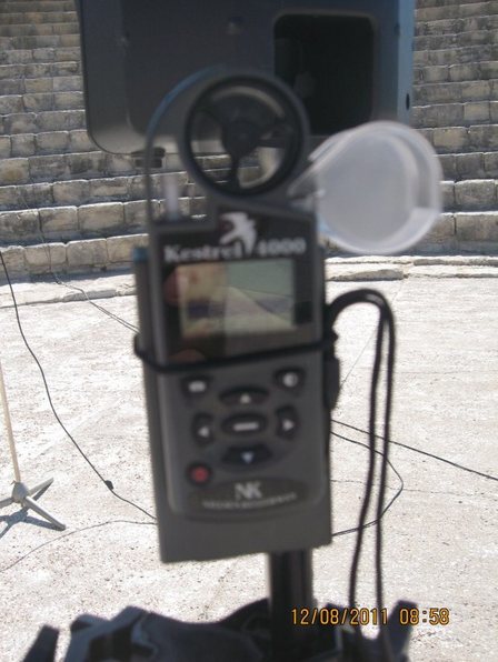
Figure 13. The portable weather station used at Kourion theatre.
Results
The results of Kourion measurements are shown below in terms of Excess Attenuation (EA) versus frequency and EA versus distance. Excess Attenuation was used in the presentation of results since sound pressure levels are biased by sound source and microphone response. For EA analysis the sound measurements were corrected for distance attenuation. In all simulations, 2nd order reflections were used, the maximum order detected by OTL – Terrain for all 35 receivers and a 2nd order sound diffraction. The analysis was carried out in 1 Hz resolution between 50 and 10000 Hz. A third party commercial software was used with the semicircular geometry as a model to verify that only 2nd order reflections are possible in the theatre.
The results of Kourion measurements are shown below in terms of Excess Attenuation (EA) versus frequency and EA versus distance. Excess Attenuation was used in the presentation of results since sound pressure levels are biased by sound source and microphone response. For EA analysis the sound measurements were corrected for distance attenuation. In all simulations, 2nd order reflections were used, the maximum order detected by OTL – Terrain for all 35 receivers and a 2nd order sound diffraction. The analysis was carried out in 1 Hz resolution between 50 and 10000 Hz. A third party commercial software was used with the semicircular geometry as a model to verify that only 2nd order reflections are possible in the theatre.
EA vs Frequency – results of measurements and simulations with and without 2nd order diffraction effects.
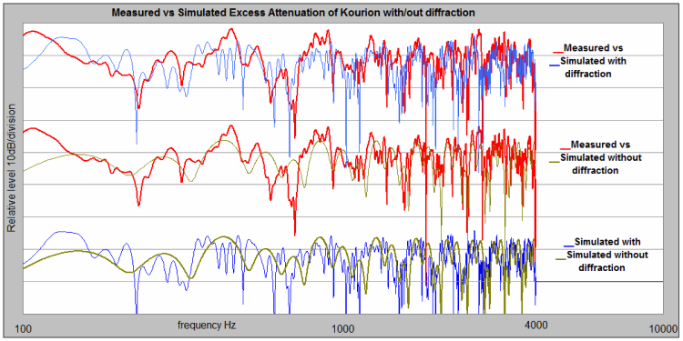
Figure 14. EA results extracted from Kourion measurements, compared to simulation results, with and without diffraction, in relative levels
EA vs Frequency - results of measurements and simulations with 2nd order diffraction effects, at three steps.
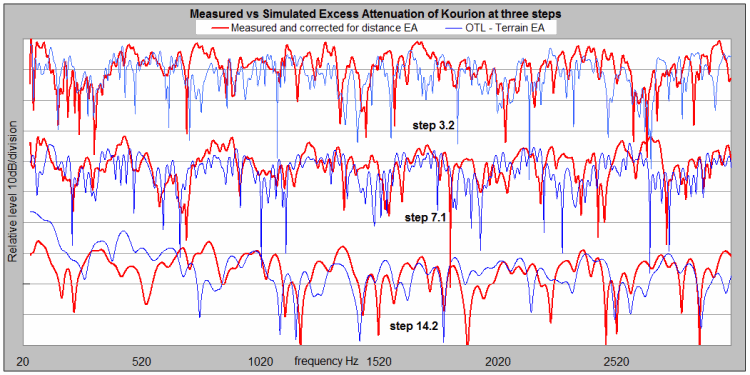
Figure 15. Sound measurements and simulation results with 2nd order diffraction at three Kourion steps, 3rd, 7th, 14th, out of total of 17.
EA vs Distance
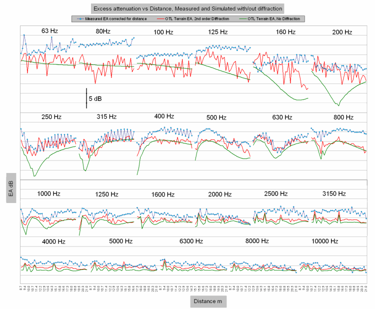
Figure 16. EA against distance (at intervals of 38.5 cm) in 1/3rd octave bands. Sound measurements versus simulation results with and without diffraction.
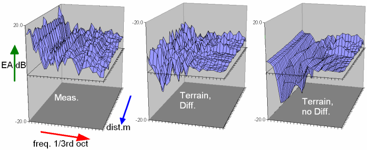
Figure 17. Excess Attenuation results versus distance and frequency (in 1/3rd oct. bands). Left - measured, middle - simulated with diffraction, right - simulated without diffraction.
Conclusions
- Sound predictions and simulations could come close to real life sound fields provided they include sound diffraction effects. Simulations with sound diffraction in high frequency resolution analysis provide the finer structure of sound fields.
- For engineering purposes, 1/3rd or 1/1 octave bands might be adequate, however, for sound analysis purposes, a high resolution analysis is compulsory.
- The study of open spaces such as ancient theatres by the method of simulation is much more demanding than closed spaces since acoustical effects are more evident due to the non returning waves escaping into the environment.
- Sound diffraction enhances sound diffusion and has a greater effect on low rather than high frequencies.
Ray Equivalency Theorem
Ray Equivalency Theorem
Theorem
Assuming a circular curve C with central angle < π, a line L crossing the plane of C perpendicularly at the center of C, a point P on L and a point O not on L, there is only one diffraction ray connecting C, P and O, crossing C at point F (First claim). This ray is equivalent to the diffraction ray connecting the tangent at F, P and O (Second claim).
Assuming a circular curve C with central angle < π, a line L crossing the plane of C perpendicularly at the center of C, a point P on L and a point O not on L, there is only one diffraction ray connecting C, P and O, crossing C at point F (First claim). This ray is equivalent to the diffraction ray connecting the tangent at F, P and O (Second claim).
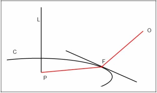
Figure 1. Ray Equivalency Theorem
Axioms
- Each diffraction ray is the shortest ray connecting a source, an edge and a
receiver. - Angle of incidence of a diffracted ray on an edge is equal to the angle of
diffraction. - The angle of incidence of any radius on the perimeter of a circle is 90o.
- Assuming a circular curve C with central angle <π, a line L crossing the plane of
C perpendicularly at the center of C, for any point P that is not on L there is only
one tangent T on C where the angle between P, the projection of P on T (PP) and
any point on T not equal to PP is equal to 90o.
Proof
Since 3 is true then the angle of incidence of any diffracted ray on C will be 90o. Since 4 is true then there is only one ray that can have an angle of diffraction equal to 90o. Since 2 is true then there is only one diffracted ray that can satisfy this condition. This proposition proves the first claim of the theorem.
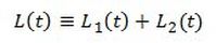
The second claim can be proved as follows. The length of a diffracted ray can be written as
Since 3 is true then the angle of incidence of any diffracted ray on C will be 90o. Since 4 is true then there is only one ray that can have an angle of diffraction equal to 90o. Since 2 is true then there is only one diffracted ray that can satisfy this condition. This proposition proves the first claim of the theorem.
The second claim can be proved as follows. The length of a diffracted ray can be written as
|
Eq. 1
|
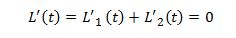
Where t is a parameter that varies over some interval I. I implies a movement of unit length along the curve. We are interested in finding t in the interior of I that minimizes t. The necessary condition for such t is a differential condition that may be written
|
Eq. 2
|
Since Eq. 2 is an equation that has differential conditions, then the conditions that determine a diffraction point depend on the nature of the curve C only in a local neighborhood. As a corollary, we see the following. Any diffraction point x on C, is a diffraction point on the straight line that is tangent C at x.